Generalizing The QR System
The Embedded QR code system so far has been outlined in terms of pipeline, but it always relies on the assumption that all images will behave as the lena image, which as a fact, is not true. So the next step is to generalize the system to work with any image.
The different constants used so far are:
-
Squared host image
-
Uses QR image size and resizes host to it.
-
Guassian noise constants:
-
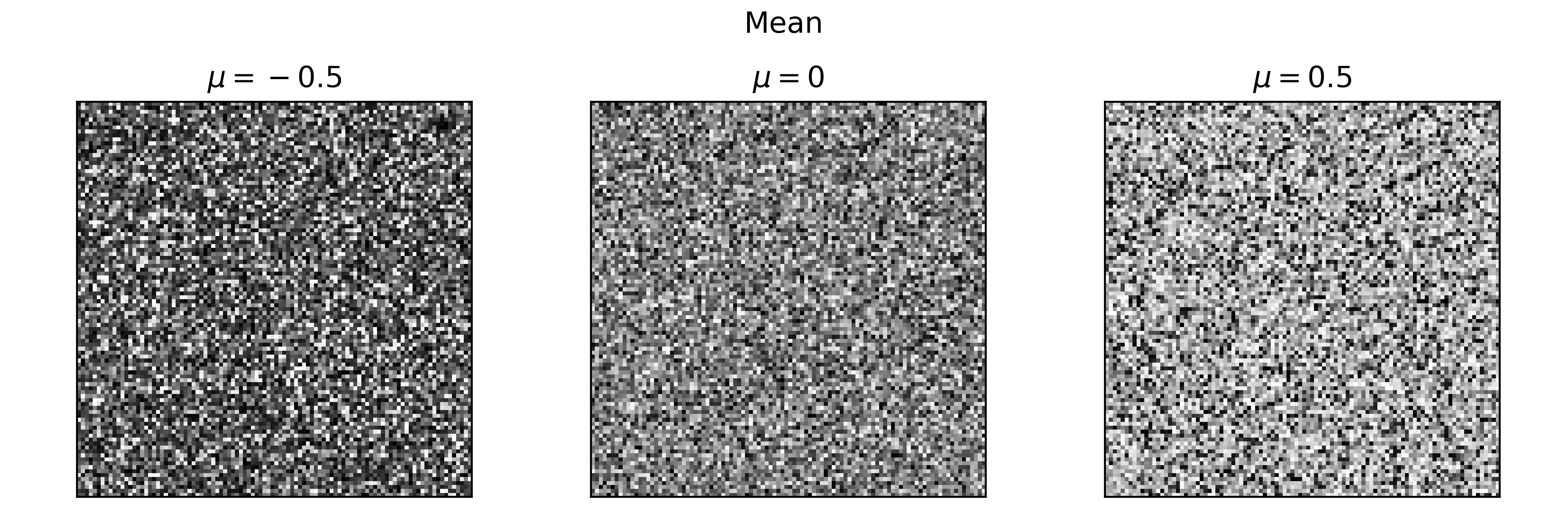
Mean = 0. Conclusion: always 0
The function to create a gaussian noise image is:
  def gaussian_noise_2d(mean, stdev, size):
  gauss = np.random.normal(mean, stdev, (size[0], size[1]))
  gauss = gauss.reshape(size[0],size[1])
  # (-1,1) to (0,1)
  gauss = 0.5 * (gauss + 1.0)
  # (0,1) to (0, 255)
  gauss = (gauss * 255).astype('uint8')
  return gauss
The
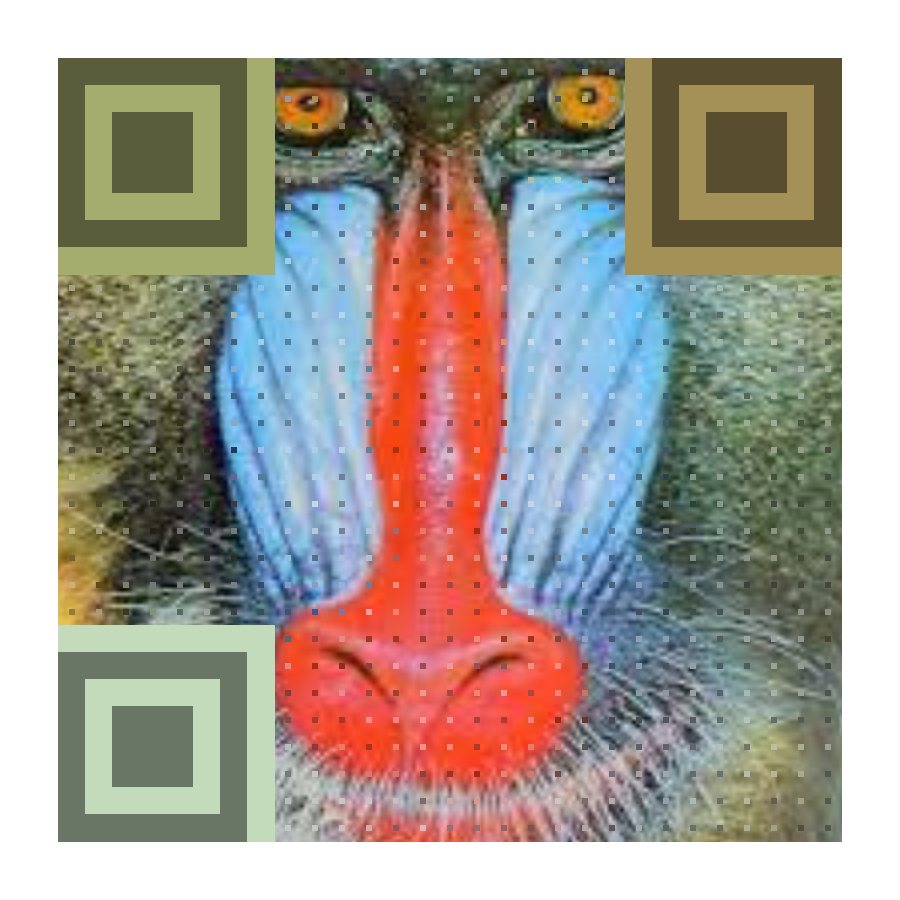
np.random.normal(loc, scale, size)defines aslocthe center of the distribution, around which the 68% of all randoms generated will fall into. We defined mean = 0 in the proof of concept program, and then all those numbers are generated in a range [-1, 1], centered at mean = 0. Then, the array gets moved to a domain of range [0, 1], meaning the center is now at 0.5 or 127 in a scale of 0 to 255. From this, we can conclude that for the general program, and for any host image, the center or mean of the gaussian noise must be $\mu = 0$.The following image shows the results from shifting $\mu$ to values -0.5, 0 and 0.5, and keeping a standard deviation of $\sigma = 0.5$.
-
Std dev = 0.5. Conclusion: always 0.5
The
np.random.normal(loc, scale, size)defines asscalethe standard deviation of the distribution, that is, the speard or width of the gaussian bell. The standard deviation is the square root of the variance, and thus we are eliminating the sign of the differences of the numbers in the dataset with the mean, because we only care about its distance to the center. The mayority of data is within the range of $[\mu - \sigma, \mu + \sigma]$. We say the mayority instead of a percentage because the exact percentage depends on the distribution that the data has. For example, if it was a normal distribution we would say that the 68% of data points are within the range mentioned.In the proof of concept program we used a standard deviation of $\sigma = 0.5$, and by following the function for the gaussian noise above, we can say that the 68% of the data points are 0.5 units from the center 0. With the first domain shift, this becomes 0.25 from the center at 0.5; with the second domain shift, this becomes 64 units from the center at 127. Thus, 68% of the data points lie in a range of [127-64, 127+64]. Since this is the range of color in RGB (0 to 255), the $\sigma = 0.5$ for the gaussian noise must stay the same for all cases.
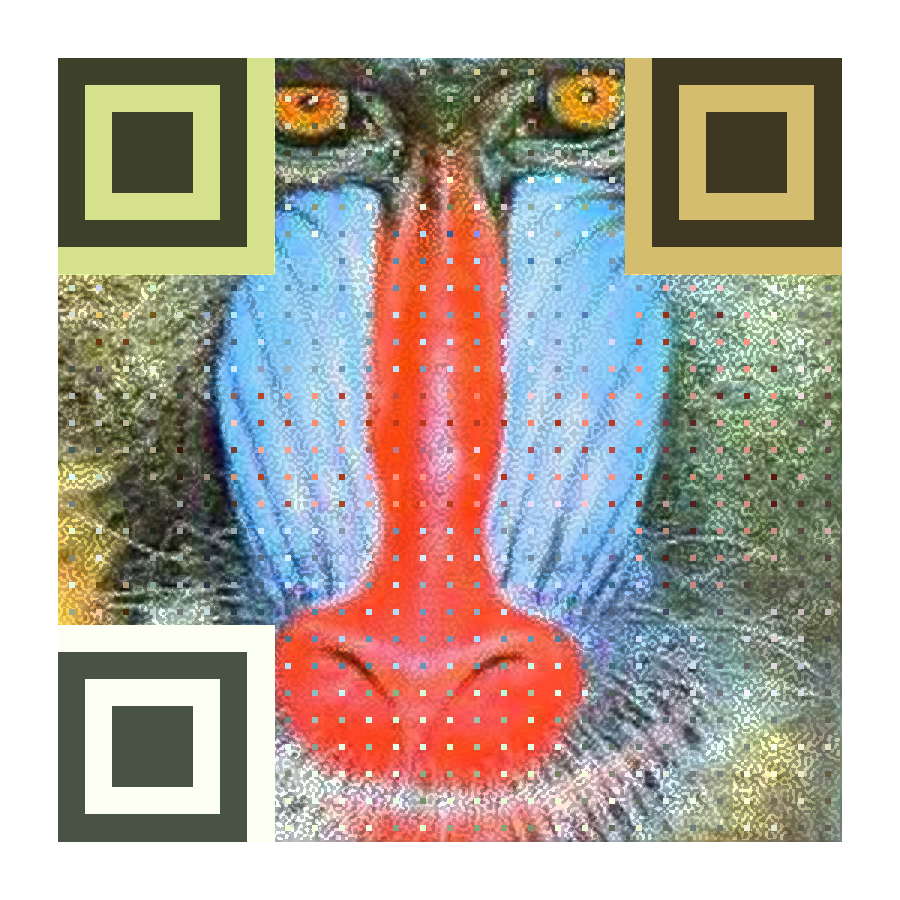
The following image shows the results from shifting $\sigma$ to values 0.25, 0.5 and 0.75, and keeping a mean of $\mu = 0$.
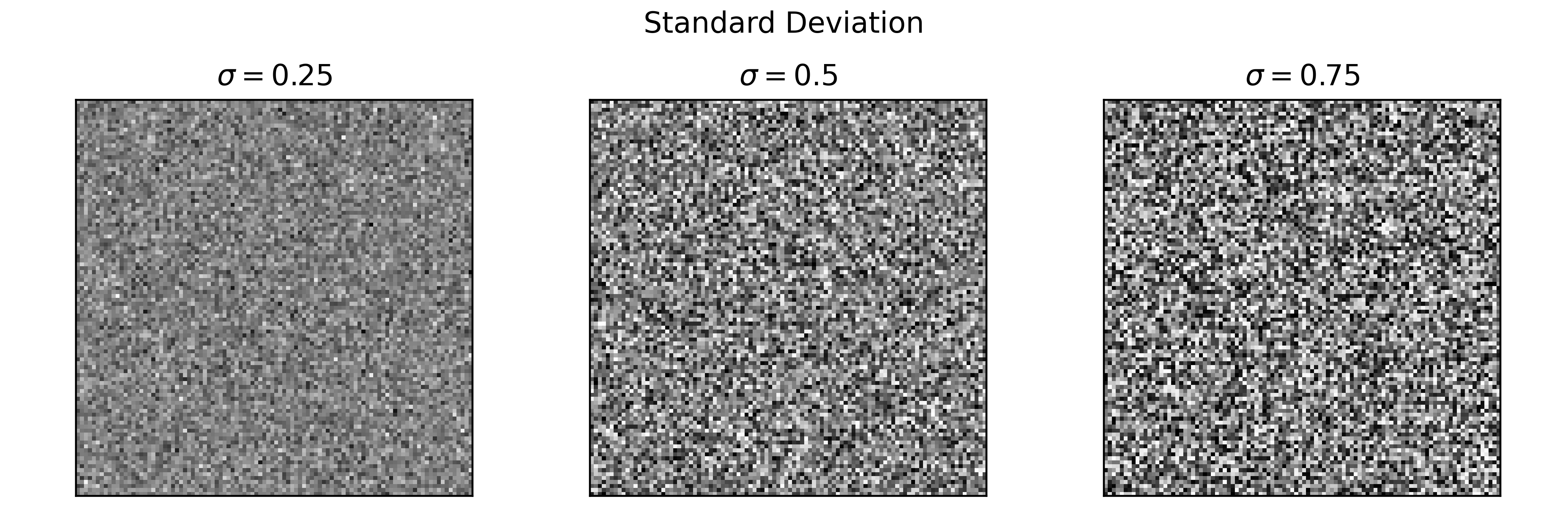
We see that in the first case the distance to the center (127) is the smallest, which means that the majority (68%) of the points are very near the gray with value 127. That’s why we see not so many variation in tones, meaning there’s not much contrast. For larger deviations or distances to the center, we see more variation, more contrast.
-
-
Blue noise constants:
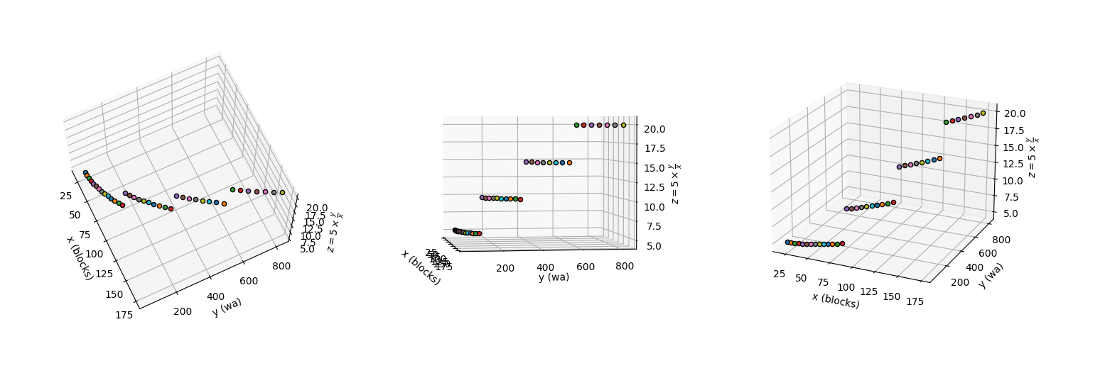
- Iterations: 5. Conclusion: i = 5*(wa / blocks)
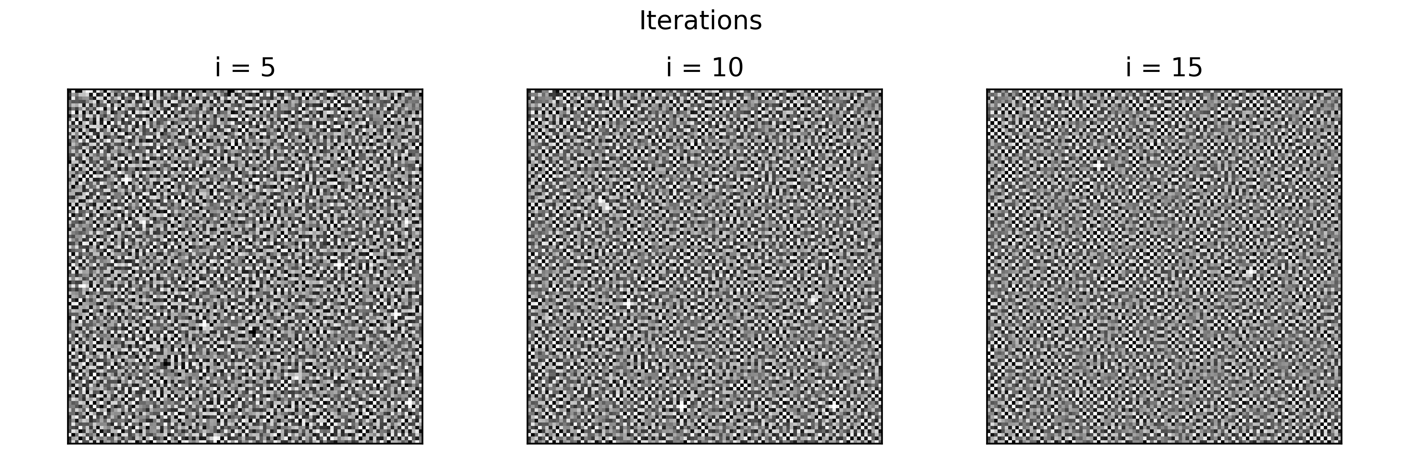
Blue noise is basically high frequency noise. To get the high frequency values of white noise, we blur the image and substract that image to the original. This can be done multiple times, and thus we defined a value for iterations.
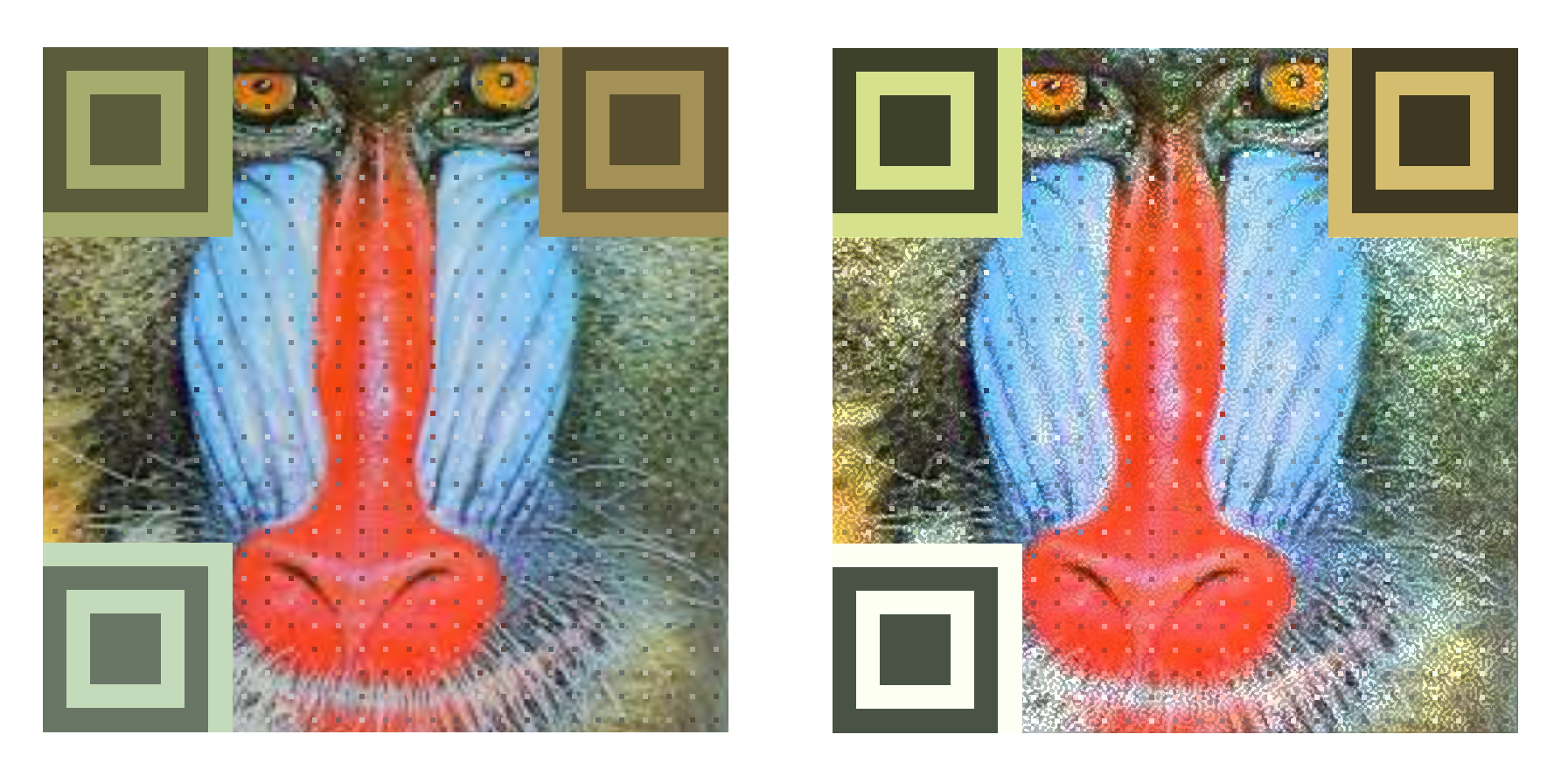
  def blue_noise(iterations, sigma, inputImg):
      for i in range(iterations):
          # high pass filter: low pass filter it, subtstract that from the original image
          high_pass = highpass(inputImg, sigma)
          # normalize the histogram
          norm = normalize_histogram(high_pass)
          inputImg = norm
      return inputImg
The more iterations, the blurrier the original image gets, and this in turn makes the substraction larger and larger, because a blurried image (almost gray) has larger differences to a sharp white noise. This generates the image below, where we can see that the more iterations, the more dense the noise pattern gets, as if the image slowly gets more similar to white noise (?).
We will use a simple heuristic: $i = 5 \times \frac{w_a}{blocks}$, where $i$ is the iterations variable. Since the initial value is 5 iterations for a 29-block QR with each module being around 27 pixels, then this function will still output 5 for that case, and the iterations wouldnt increase that easily unless the blocks reach a large number, which means the QR is quite dense and the noise pattern needs to be so as well. This can be seen below.
- Sigma: 0.8. Conclusion: always 0.8
As we discussed in the standard deviation of the white noise pattern, the standard deviation maintains the contrast. In this case, this sigma is used for the gaussian blur, and thus defines the ‘gray’ levels for the blur effect. This can be kept as a constant.
-
Overlay mask alpha: 0.2. Conclusion: always 0.2
This mask, although not mentioned much in the algorithm, is used to compute the average RGB tone so that with the computer sub-window averages we can modify (decrease or increase) the color of the $w_a \times w_a$ area. This might stay as a constant for now.
-
Factor to increase/decrease from average luminance + rgb: 0.3
-
$\beta$, $\alpha$, $\beta_{c}$ and $\alpha_c$. These are for the non-center module pixels.
System Fixes
General Issues
- The first major bug I have just bumped into is the fact that the python system outputs the following (look at the modules):
while the C++ system seems to differ and actually seems to be far from the corresponding average tone:
Update: it seems fixed now. The problem was that the RGB input for the modules were taking coordinates (j, i) instead of (i, j). Human error. They look similar in tone now (look at the mdoules only):
-
Figure out what length of url is ideal, so that finder pattern colors are not needed, since they slow down decoding.
-
Then, try to optimize the HSV conversions, maybe store a global variable with the HSV image to stop calling the function over and over.
Image Processing for Ideal Input
For the calculation of the average luminosity and standard deviation, the image is converted to HSV color space and then the average and deviation is computed on the V channel.
| Image | Average | Stdev |
|---|---|---|
| Lena | 180.40 | 48.94 |
| Monkey | 157.4 | 55.45 |
| Train | 49.36 | 78.65 |
| Train (gamma corr) | 103.72 | 65.14 |
| Overexposed | 247.21 | 14.69 |
| Overexposed (gamma corr) | 208.24 | 69.97 |
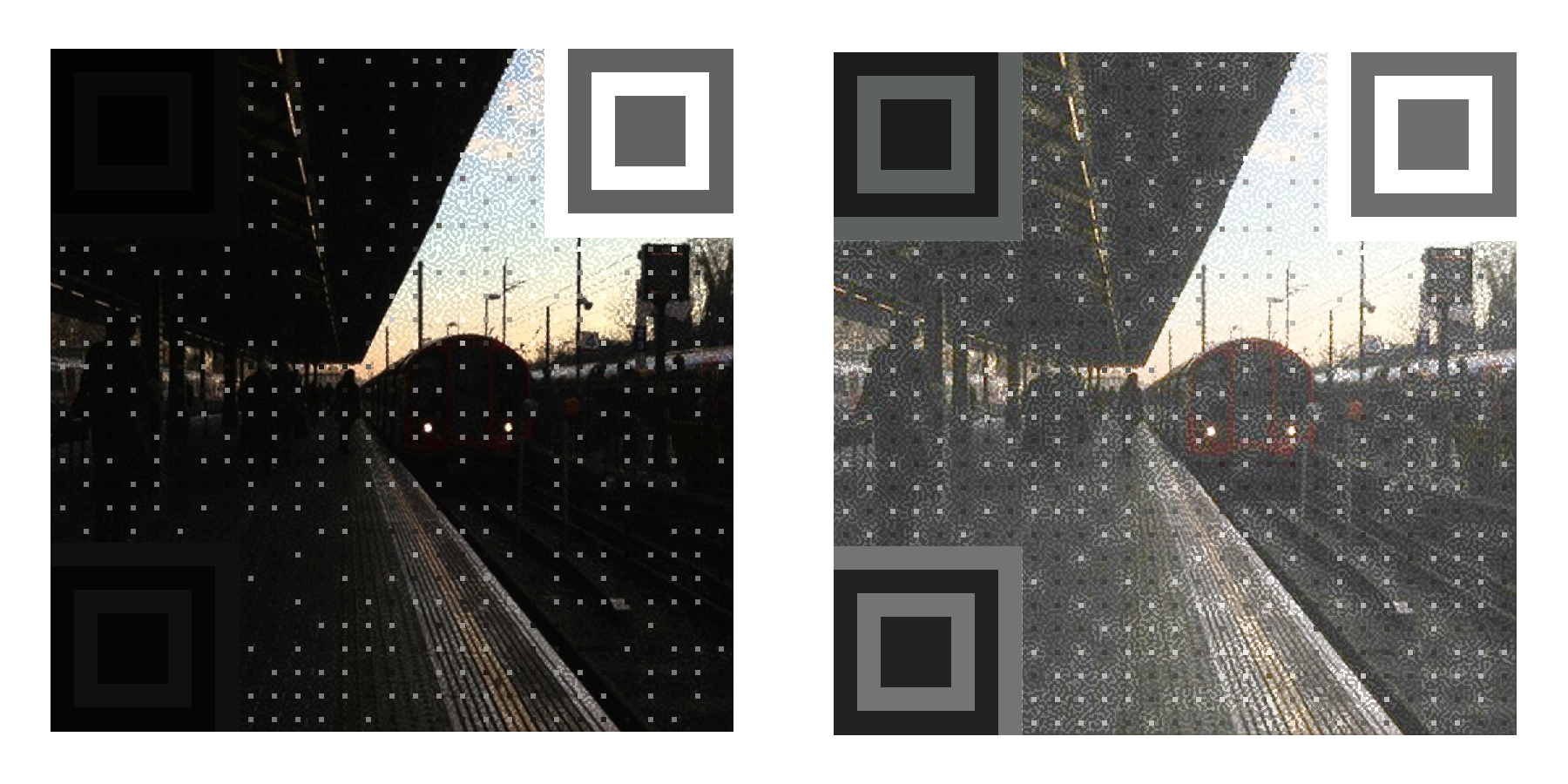
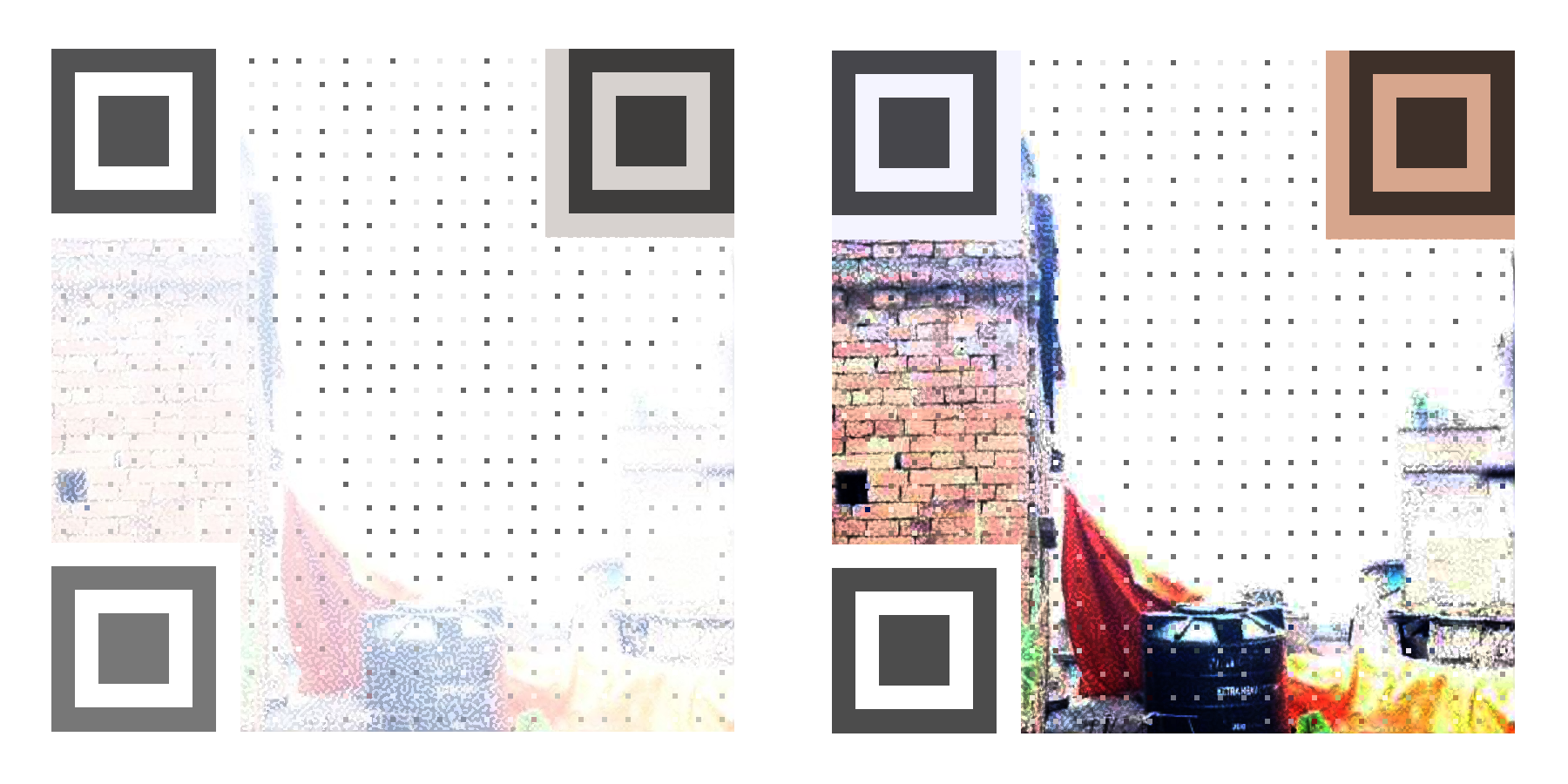
After performing a Gamma correction on the Train image, the new average is over 100, and the code results quite scannable:
The gamma correction factor is 0.4. Gamma correction can be used to correct the brightness of an image by using a non linear transformation between the input and output values:
\[O = (\frac{I}{255})^{\gamma} \times 255\]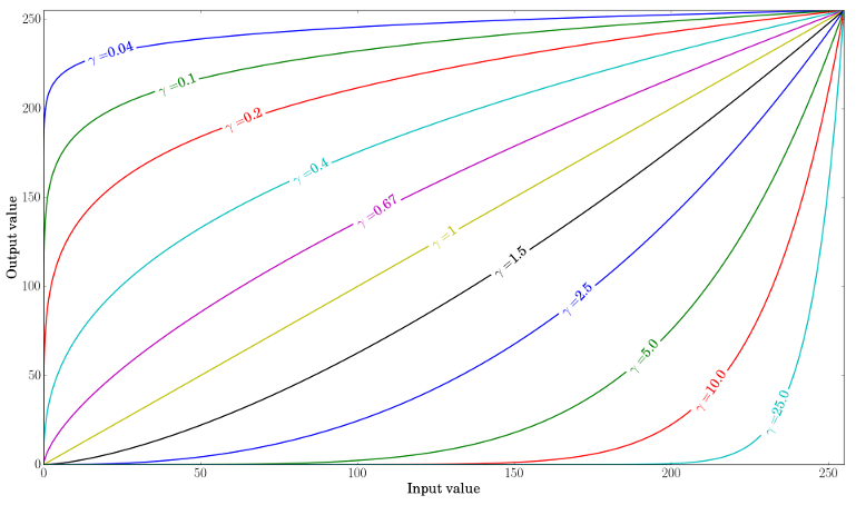
When $\gamma \lt 1$, the dark regions will be brighter and the histogram is shifted to the right.
The opposite case can also be corrected with gamma function. A 10 gamma value is used to go from the left to right image.
Therefore, the question is how to calculate the proper gamma value given any image, either underexposed, overexposed, or even a logo? Here is a discussion where they propose to do it based on the mean color in the image (which seems the most obvious) using the function:
\[\gamma(\mu) = \frac{log(127)}{log(\mu)}\]where $\mu$ is the mean color mentioned. Such model is visualized as:
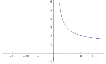
Gives an idea on how to start, but this plot gives out smaller numbers of gamma the larger the mean is; this means that the clearer the image is, the smaller the gamma is. But, as we saw in the two extreme cases above, the function should go in the opposite direction: the brighter the image is (large mean), the bigger the gamma results are. Additional patterns were found: if an image has a mean in the range $100 \leq \mu \leq 200$, then there should be no processing ($\gamma = 1$), but values smaller than 100 should ascend from a range $0 \leq \gamma < 1$, and values greater than 200 should also ascend but quicker in a range of $1 <\gamma \leq 25$. Something along this sketch:
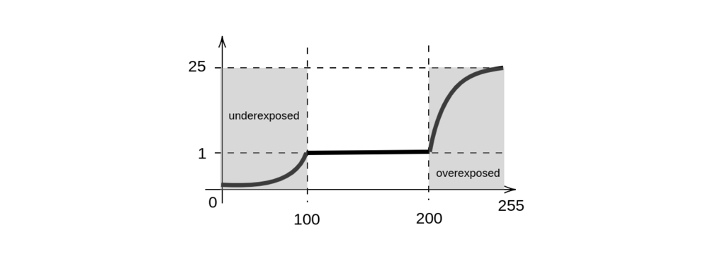
We therefore need 2 functions: one to get the gamma value when the mean is $\mu < 100$ or underexposed, and the other one to get the gamma value when the mean is $\mu > 200$ or overexposed. The middle case is when the image has a mean $100 \leq \mu \leq 200$, in which case the gamma value is 1 (no correction).
For the first part, we can get an approximation with an exponential function. But since the exponential function increases abruptly rather than smoothly, the parabola was chosen instead.
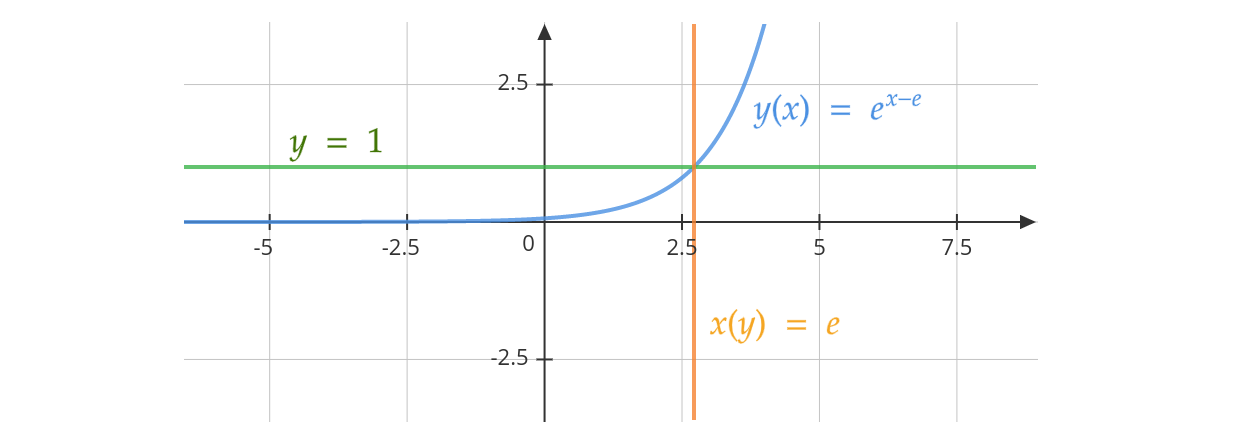
The function that fulfills the cases was found to be approximately:
\[y(\mu) = \begin{cases} \frac{\mu^2}{10000} & 0 \leq \mu < 100 \\ 1 & 100 \leq \mu \leq 200 \\ 3e\log\left(\mu-200\right)+4e & 200 < \mu \leq 255 \end{cases}\]The first and third equations are plotted below. For the third one it was difficult to find a function with an exact intersection at (255, 25), but a logarithm gives an approximation to the desired intersections and curve shape.
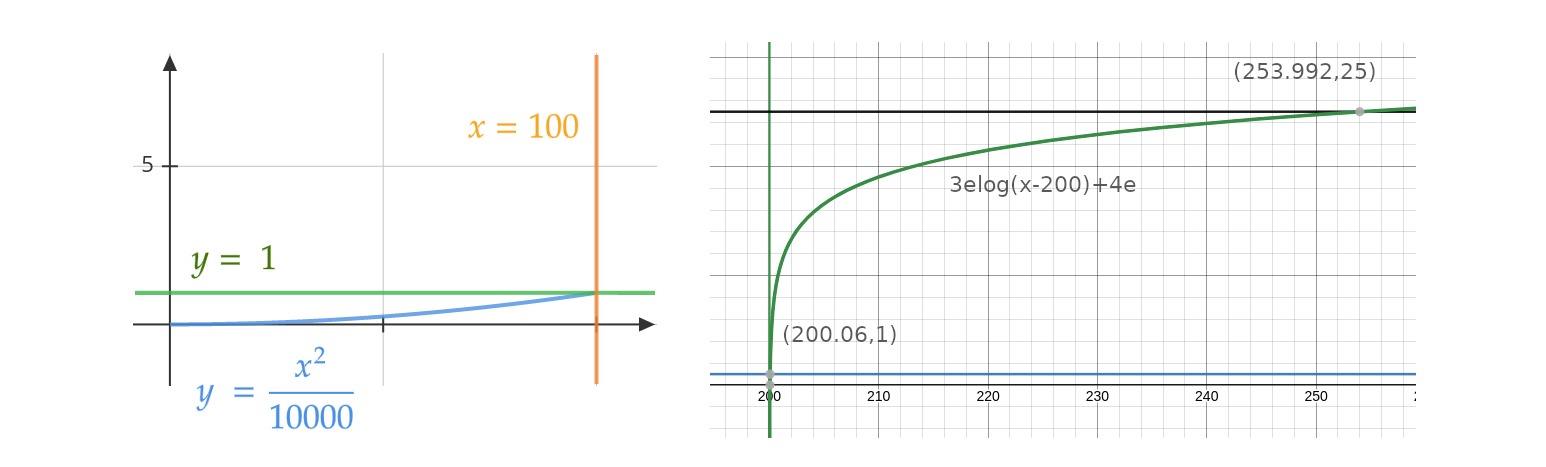
Important: log in this case refers to logarithm base 10.
Well, the underexposed values were too close to zero most of the cases, so the function was shifted by 25% in the y axis, which means that it now hits the point (0, 0.25) and its limit is (100, 1.0005) $\approx$ (100, 1.0005).
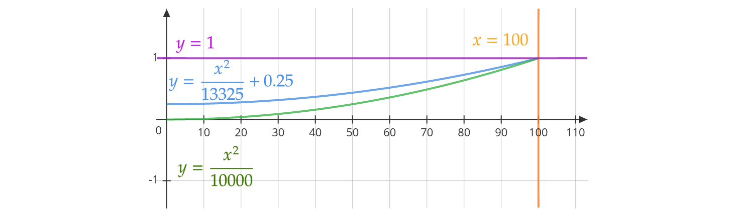
Therefore, the gamma factor is given by this function:
\[y(\mu) = \begin{cases} \frac{\mu^2}{13325}+\frac{1}{4} & 0 \leq \mu < 100 \\ 1 & 100 \leq \mu \leq 200 \\ 3e\log\left(\mu-200\right)+4e & 200 < \mu \leq 255 \end{cases}\]References
-
https://mathematica.stackexchange.com/questions/57389/convert-spectral-distribution-to-rgb-color
-
https://www.fourmilab.ch/documents/specrend/
-
Video processing idea: https://mathematica.stackexchange.com/questions/60292/how-to-build-a-bvh-a-motion-capture-file-format-player-in-mathematica/60942#60942
-
user: https://mathematica.stackexchange.com/users/57/sjoerd-c-de-vries
-
equalize: https://stackoverflow.com/questions/15007304/histogram-equalization-not-working-on-color-image-opencv
-
gamma: https://docs.opencv.org/3.4/d3/dc1/tutorial_basic_linear_transform.html
-
color quantization: https://en.wikipedia.org/wiki/Color_quantization
-
color classification: https://stackoverflow.com/questions/11411889/color-classification-with-k-means-in-opencv/
-
detect underexposed image opencv c++
-
https://stackoverflow.com/questions/11562048/how-can-i-find-a-good-image-on-the-base-of-a-histogram
-
https://codereview.stackexchange.com/questions/284179/proper-implementation-of-signal-handler-and-multithreading-pthread
-
the best gamma correction: https://stackoverflow.com/questions/61695773/how-to-set-the-best-value-for-gamma-correction
-
https://stackoverflow.com/questions/61695773/how-to-set-the-best-value-for-gamma-correction
-
user: https://stackoverflow.com/users/7355741/fmw42
-
user: http://www.fmwconcepts.com/fmw/fmw.html
-
metamerism: http://simonstechblog.blogspot.com/