Thoughts On Metamerism
Metamers are stimuli with divergent spectral power distributions that have the same color and luminance. Metamers achieve this effect because each of the human cone photoreceptors responds to the total light across a wide range of wavelengths, weighted according to their spectral sensitivity (Allen et al., 2018). Metamers are color stimuli which, although they differ in wavelength composition, look alike in hue, saturation, and brightness to an observer. Metamers look alike because they excite the visual receptor system in exactly the same way, evoking the same balance of stimulation across the several receptor types (Cohen et al., 1982).
Thus metamers can serve as substitutes for one another, and in most color-matching operations one achieves metameric matches, not exact matches in stimulus wavelength composition (Cohen et al., 1982). Hence these colors can be described by their three-color metamers, and a generalized procedure of colorstimulus specification by a system of tristimulus values becomes possible. Tristimulus values for any stimulus can be calculated from the spectral energy distribution of that stimulus by referring to tabled data from experiments in which wavelength segments have been matched by levels of three chosen primaries.
It is possible to make changes in the intensity and wavelength of light without altering the effective photon flux. This concept is employed by RGB (Red, Green, Blue) displays to recreate realistic images using a spectral composition that is very different from that of the real world. This allows modulation of subconscious/reflex light responses amplitude without changing visual appearance.
Two metameric color stimuli have spectral-power-distribution curves which, in general, intersect at three or more wavelengths within the visible spectrum (Ohta et al., 1977). One of these wavelengths is located in the short-wavelength region, one in the middle-wavelength region, and one in the longwavelength region. Recent work by Thornton puts these wavelengths at 448 $\pm$ 4 nm, 537 $\pm$ 3 nm, and 612 $\pm$ 8 nm, respectively. These regions correspond to the regions in which the “blue,” “green,” and “red” spectral-response functions of our visual system are respectively predominant. We will call the points of intersection the nodes of metameric color stimuli. In between the nodes there are the loops.
I found a post in Pete Shirley’s Blog titled The blue dress illusion, where he explains that the difference in perception regarding the color of the dress is due to the light surrounding it and posts an image he found on Twitter:
This is the same concept illustrated in my copy of The Structure and Properties of Color Spaces and the Representation of Color Images by Eric Dubois. This makes me think that exploring the idea of creating a metameric color that gives the illusion of it being not very constrasting to the QR image but being so in numerical terms, not so crazy.
Color Rendering of Spectra
Following a post written by John Walker, once the spectrum of the light impinging upon a point in the image plane is known, the eye’s perception of that spectrum must be determined. Display arguments must be calculated which evoke that perception in the viewer. First we developed a script that, given light with an arbitary spectrum, determines the CIE X, Y and Z values which characterize a standard human observer’s perception of its colour, then calculates their corresponding RGB values for display.
We define a spectrum as a function $P(\lambda)$ which gives, for any wavelength $\lambda$ in the human visual range of 380 through 780 nanometres (nm), the power emitted per small constant-width wavelength interval centred about $\lambda$, normally in units of watts per nm.
Emission spectra of light sources and transmission, reflection, and absorption spectra of materials are usually determined empirically by spectrophotometry and specified in a table of measurements at wavelength intervals, normally 5 nm, throughout the visual range.
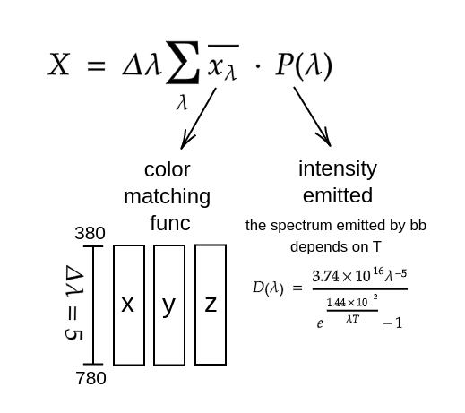
The CIE Color matching functions, $\bar{x}(\lambda), \bar{y}(\lambda), \bar{z}(\lambda)$ represent the relative contributions of light with wavelength $\lambda$ to the CIE tristimulus values X, Y and Z. The color matching functions were determined by measuring the mean color perception of a sample of human observers over the visual range from $\lambda_{violet} = 380$ to $\lambda_{red} = 780$ nm. To compute CIE X, Y and Z values for light with spectrum $P(\lambda)$ we sum the products of the color matching function weights at each wavelength (380 to 780 nm) and the intensity emitted at a constant narrow wavelength interval centered at that $\lambda$.
\[X = \delta \lambda \sum_{\lambda = \lambda_{red}}^{\lambda_{violet}} \bar{x_{\lambda}} \cdot P(\lambda),\] \[Y = \delta \lambda \sum_{\lambda = \lambda_{red}}^{\lambda_{violet}} \bar{y_{\lambda}} \cdot P(\lambda),\] \[Z = \delta \lambda \sum_{\lambda = \lambda_{red}}^{\lambda_{violet}} \bar{z_{\lambda}} \cdot P(\lambda).\]For most purposes sampling wavelength bands 5 or 10 nm apart is adequate, (CIE 1971) and (CIE 1986) provide color matching tables with 1 nm resolution. The table cieColorMatch in the program gives the CIE colour matching functions every 5 nm.
The CIE Y value is a measure of perceived luminosity of the light source. In rendering, we are usually interested in relative luminosities so we can ignore absolute values of Y and simply scale luminosities between min and max brightness. The X and Z components give the colour or chromaticity of the spectrum. Since the perceived colour depends (again, with the usual simplifications) only upon the relative magnitudes of X, Y, and Z, we define its chromaticity coordinates as:
\[x = \frac{X}{(X + Y + Z)},\] \[y = \frac{Y}{(X + Y + Z)},\] \[z = \frac{Z}{(X + Y + Z)}.\]Since
\[x + y + z = \frac{X + Y + Z}{X + Y + Z} = 1,\]$z$ canbe obtained from x and y:
\[z = 1 - (x + y)\]Therefore, cromacity coordinates are usually given by x and y. In the image below, we can see CIE chromacity diagram. Pure spectral colours lie on the curved border of the “tongue”, labeled by wavelength. R, G, and B are the SMPTE primaries. W marks the SMPTE white point, CIE Illuminant D65. C is a colour which can be generated by mixing R, G, and B; it is said to lie within the colour gamut they define.
If an output device accepts CIE colour specifications directly and transforms them into its colour gamut, we have nothing to compute. However, displays amd printers require device-specific colour specifications in systems such as RGB or CMYK, requiring the conversion from CIE perceptual color into device parameters.
| Red | Green | Blue | White Point | |
|---|---|---|---|---|
| System | x,y | x,y | x,y | x,y |
| NTSC | 0.67,0.33 | 0.21,0.71 | 0.14,0.08 | 0.3101,0.3162 |
| EBU (PAL/SECAM) | 0.64,0.33 | 0.29,0.60 | 0.15,0.06 | 0.3127,0.3291 |
| SMPTE | 0.630,0.340 | 0.310,0.595 | 0.155,0.070 | 0.3127,0.3291 |
The CIE Y component indicates the intensity of the light and the chromaticity coordinates x and y its colour in the CIE colour diagram. An RGB display mixes three primary colours, each of which is described by its CIE x and y (and implicitly z) coordinates. The three primaries define a triangle on the CIE diagram—any colour within it can be formed by mixing them. Table 1 lists the CIE x and y coordinates of the phosphors and reference white points of various broadcast systems. As noted in (Martindale and Paeth 1991), the NTSC primaries aren’t remotely similar to those used in modern displays. Regrettably, the specifications of RGB monitors rarely include phosphor chromaticities, so unless you’re prepared (and equipped) to calibrate the phosphors yourself, you’re forced into choosing a “reasonable” set. Martindale and Paeth recommend calibrating to the SMPTE primaries, which are close to the EBU primaries used in PAL and SECAM broadcasting.
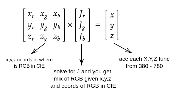
The amount of each primary to mix to yield a CIE colour with a given x, y, and z is the unknown $J$ vector in the equation:
\[\begin{bmatrix} x_r & x_g & x_b\\ y_r & y_g & y_b\\ z_r & z_g & z_b \end{bmatrix} \cdot \begin{bmatrix} J_r \\ J_g \\ J_b \end{bmatrix} = \begin{bmatrix} x \\ y \\ z \end{bmatrix}\]Solving for Jr, Jg, and Jb gives the weighting of Red, Green, and Blue primaries which yield the desired x, y, and z or, in other words, the coefficients of a linear combination of the primaries’ chromaticity coordinates. The absolute intensity may then be adjusted based on the Y component (luminosity). The linear RGB values will require gamma correction if the display device has nonlinear response (non-unity gamma).
The handling of colours unrepresentable on a given output device varies from application to application. An approach which often yields acceptable results is reducing the saturation of the requested colour until it falls within the RGB gamut. A colour outside the RGB primary triangle will thus always be more saturated than can be displayed (since the ones lying on the tongue are fully saturated), and consequently must be approximated by a less saturated colour.
The spectral composition of many light sources is complicated and must be tabulated from photometric measurements. One useful family of light sources whose spectrum can be expressed as a simple function is the Planckian or black body radiators. The spectrum emitted by an ideal black body is determined entirely by its temperature; many natural and artificial light sources can be approximated by black body radiators of various temperatures.
| Source | Temperature, K |
|---|---|
| Candle flame | 1900 |
| Sunlight at sunset | 2000 |
| Tungsten bulb—60 watt | 2800 |
| Tungsten bulb—200 watt | 2900 |
| Tungsten/halogen lamp | 3300 |
| Carbon arc lamp | 3780 |
| Sunlight plus skylight | 5500 |
| Xenon strobe light | 6000 |
| Overcast sky | 6500 |
| North sky light | 7500 |
For an ideal black body at temperature $T$ (Kelvins), the emittance at a given wavelength $\lambda$ (metres) is calculated by Planck’s radiation law:
\[P_{\lambda}d\lambda = \frac{c_1 \lambda^{-5}}{e^{\frac{c_2}{\lambda T}} - 1}\]Where $P_{\lambda}d\lambda$ is the hemispherical flux density in watts per square centimetre in the wavelength range between $\lambda$ and $\lambda + d\lambda$. Constants $c_1$ and $c_2$ are:
\[c_1 = 3.74183 \times 10^{-16} W m^2,\] \[c_2 = 1.4388 \times 10^{-2} m K\]To determine the CIE XYZ coordinates of a black body with temperature T, we use Eqs. (1) to sum, across the visual spectrum, the products of the CIE colour matching functions and the black body power spectrum from Eq. (4) (this last one). This spectrum_to_xyz which uses the function bb_spectrum that evaluates Planck’s law. We ignore the $\delta \lambda$ in the first equation, since we are only interested in the color of the black body and not its absolute luminosity.
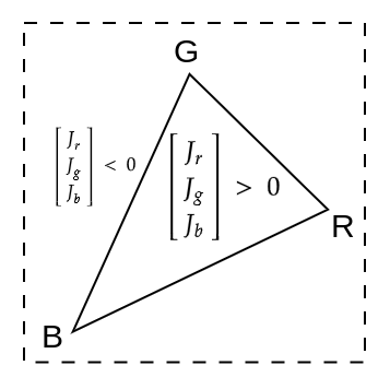
Having found the chromaticity coordinates x, y, and z, we must next convert them to RGB intensities in a chosen colour system. The function xyz_to_rgb solves Eq. (3) for all J’s, or the amount of each primary to mix. If the colour lies inside the triangle formed by the primaries, all the J weights will be nonnegative. If one of the J values is negative, the colour falls outside the RGB gamut (the negative J indicates we would have to subtract that primary to obtain the requested x, y, and z); the C function inside_gamut performs this test.
If the requested colour is outside the gamut, the function constrain_rgb replaces it with the nearest within-gamut colour by mixing it with the colour system’s white point. Finally, we print the CIE and RGB colours of a black body with the given temperature, indicating whether gamut limitations required desaturating the RGB mixture.
The realtionship between the values X, Y and Z given a temperature and its corresponding R, G and B is represented by the following plot. This is for the color system known as CIE.
Now, if we want to plot the spectrum density of one of the colors gotten from a single temperature, we need to add to the function that evaluates the first equation three arrays to store each of the values accumulated to X, Y and Z at each wavelength $\lambda$ in the visible range. Then, each X, Y and Z arrays are plotted separately.

Since the above plot was just for one of the temperatures, in order to analyse how the plot change as the RGB changes, we can store each of the X,Y and Z arrays for each of the temperatures we want, that is 19, in this case. The plot turns out as follows.
To summarize, the first thing is to have each X, Y and Z functions:
Then, we solve for $J$ vector,
Finally, we correct the RGB to fit inside the RGB gamut triangle inside the CIE diagram.
Side Note
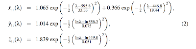
Pete Shirley’s post talks additionally about how the color matching functions (defined in our array cieColorMatch) can be prone to typos, and therefore he co-wrote a paper where they approximated the functions so that they yield the numbers on the cie color matching table functions. This is another proof of The Art of Approximation introduced to me in the lands of Croatia by Dr. Bruno Klajn.
Maybe I need to code something to get the Temperature given the RGB, so that the X,Y and Z functions can be defined. Then the metameric color is computed to intersect the X,Y and Z three times. From that, we got the metameric X, Y and Z, from which we solve for J vector, getting the RGB of the metamer, correct it and display it.
Update
It seems that with the code evaluating the temperatures from 1000K to 10001K by a step of 500K cannot output all colors in the RGB color space.
The color gamut that you get from a range of temperatures depends on the color temperature to RGB conversion formula used. However, in general, it is difficult to obtain a pure green gamut using the Planck radiation law because green is not a dominant color in the visible spectrum emitted by a blackbody at any temperature.
That being said, we can try adjusting the temperature range and step size to see if you can obtain a more green gamut. We can also try using different color temperature to RGB conversion formulas to see if they give you a better result. Some ideas:
-
Try using a narrower temperature range that is centered around the temperature range where green is most prominent in the visible spectrum. This range is typically between 5000K and 7000K.
-
Use a smaller step size between temperatures to obtain more colors in the range. A step size of 100 or 50 may give you more colors to work with.
-
Experiment with different color temperature to RGB conversion formulas. There are many formulas available, and some may give you better results for a green gamut. For example, you can try the sRGB or Adobe RGB color spaces, or use a more recent standard such as Rec. 2020.
References
(Allen et al., 2018) Allen, A. E., Hazelhoff, E. M., Martial, F. P., Cajochen, C., & Lucas, R. J. (2018). Exploiting metamerism to regulate the impact of a visual display on alertness and melatonin suppression independent of visual appearance. Sleep, 41(8), zsy100.
(Cohen et al., 1982) Cohen, J. B., & Kappauf, W. E. (1982). Metameric color stimuli, fundamental metamers, and Wyszecki’s metameric blacks. The American journal of psychology, 537-564.
(Ohta et al., 1977) Ohta, N., & Wyszecki, G. (1977). Location of the nodes of metameric color stimuli.
-
https://mathematica.stackexchange.com/questions/57389/convert-spectral-distribution-to-rgb-color
-
https://www.fourmilab.ch/documents/specrend/
-
https://academo.org/demos/wavelength-to-colour-relationship/
-
V formula (L inspired): http://psgraphics.blogspot.com/2014/08/rgb-luminance-revisited.html
-
the color of a black body