Text Summarizing
The automatization of text summaries allows people to ‘read’ faster, especially when browsing for a text that fulfills their interests. Thus, teaching the computer how to provide a summary of a large text seems like a task that would help people find what they’re looking for faster.
Types of text summarization:
- Extraction-based summarization
In extraction-based summarization, a subset of words that represent the most important points is pulled from a piece of text and combined to make a summary.
In machine learning, extractive summarization usually involves weighing the essential sections of sentences and using the results to generate summaries.
- Abstraction-based summarization
Advanced deep learning techniques are applied to paraphrase and shorten the original document, just like humans do.
Since abstractive machine learning algorithms can generate new phrases and sentences that represent the most important information from the source text, they can assist in overcoming the grammatical inaccuracies of the extraction techniques.
How to perform text summarization?
Extraction-based summarizing
Here’s a sample text:
“Peter and Elizabeth took a taxi to attend the night party in the city. While in the party, Elizabeth collapsed and was rushed to the hospital. Since she was diagnosed with a brain injury, the doctor told Peter to stay besides her until she gets well. Therefore, Peter stayed with her at the hospital for 3 days without leaving.”
- Convert the paragraph into sentences
- The best way of doing the conversion is to extract a sentence whenever a period appears.
- Text processing
Let’s do text processing by removing the stop words (extremely common words with little meaning such as “and” and “the”), numbers, punctuation, and other special characters from the sentences.
Basic text processing:
-
Text cleaning for de-noising the text with nltk library’s set of stopwords (words that add no value to the text as they appear in most texts, ie, “that”, “the”, etc).
-
The PorterStemmer algorithm, which reduces words into their root form, ie, “cleaning” and “cleaned” becomes “clean”.
- Tokenization
Tokenizing the sentences is done to get all the words present in the sentences. Here is a list of the words:
['peter','elizabeth','took','taxi','attend','night','party','city','party','elizabeth','collapse','rush','hospital', 'diagnose','brain', 'injury', 'doctor','told','peter','stay','besides','get','well','peter', 'stayed','hospital','days','without','leaving']
- Evaluate the weighted occurrence frequency of the words
To achieve this, let’s divide the occurrence frequency of each of the words by the frequency of the most recurrent word in the paragraph, which is “Peter” that occurs three times.
| WORD | FREQUENCY | WEIGHTED FREQUENCY |
|---|---|---|
| peter | 3 | 1 |
| elizabeth | 2 | 0.67 |
| took | 1 | 0.33 |
| taxi | 1 | 0.33 |
| attend | 1 | 0.33 |
| night | 1 | 0.33 |
| party | 2 | 0.67 |
| city | 1 | 0.33 |
| collapse | 1 | 0.33 |
| rush | 1 | 0.33 |
| hospital | 2 | 0.67 |
| diagnose | 1 | 0.33 |
| brain | 1 | 0.33 |
| injury | 1 | 0.33 |
| doctor | 1 | 0.33 |
| told | 1 | 0.33 |
| stay | 2 | 0.67 |
| besides | 1 | 0.33 |
| get | 1 | 0.33 |
| well | 1 | 0.33 |
| days | 1 | 0.33 |
| without | 1 | 0.33 |
| leaving | 1 | 0.33 |
- Substitute words with their weighted frequencies
Let’s substitute each of the words found in the original sentences with their weighted frequencies. Then, we’ll compute their sum.
Since the weighted frequencies of the insignificant words, such as stop words and special characters, which were removed during the processing stage, is zero, it’s not necessary to add them.
| SENTENCE | ADD WEIGHTED FREQUENCIES | SUM | RESULT |
|---|---|---|---|
| 1 | Peter and Elizabeth took a taxi to attend the night party in the city | 1 + 0.67 + 0.33 + 0.33 + 0.33 + 0.33 + 0.67 + 0.33 | 3.99 |
| 2 | While in the party, Elizabeth collapsed and was rushed to the hospital | 0.67 + 0.67 + 0.33 + 0.33 + 0.67 | 2.67 |
| 3 | Since she was diagnosed with a brain injury, the doctor told Peter to stay besides her until she gets well. | 0.33 + 0.33 + 0.33 + 0.33 + 1 + 0.33 + 0.33 + 0.33 + 0.33 +0.33 | 3.97 |
| 4 | Therefore, Peter stayed with her at the hospital for 3 days without leaving | 1 + 0.67 + 0.67 + 0.33 + 0.33 + 0.33 | 3.33 |
From the sum of the weighted frequencies of the words, we can deduce that the first sentence carries the most weight in the paragraph. Therefore, it can give the best representative summary of what the paragraph is about.
Furthermore, if the first sentence is combined with the third sentence, which is the second-most weighty sentence in the paragraph, a better summary can be generated.
Abstraction-based summarizing
Text summarization in NLP is treated as a supervised machine learning problem. Here’s the basic pipeline:
-
Introduce a method to extract the merited keyphrases from the source document. For example, you can use part-of-speech tagging, words sequences, or other linguistic patterns to identify the keyphrases.
-
Gather text documents with positively-labeled keyphrases. The keyphrases should be compatible to the stipulated extraction technique. To increase accuracy, you can also create negatively-labeled keyphrases.
-
Train a binary machine learning classifier to make the text summarization. Some of the features you can use include:
-
Length of the keyphrase
-
Frequency of the keyphrase
-
The most recurring word in the keyphrase
-
Number of characters in the keyphrase
-
-
Finally, in the test phrase, create all the keyphrase words and sentences and carry out classification of them.
Alexander et al. proposes an attention-based encoder-decoder method, which has been used in sequence to sequence models where the decoder extracts information from the encoder based on the attention scores on the source-side information.
However, the summary can suffer from repetition and semantic irrelevance with the attention transformer architecture. Junyang Lin et al. propose to implement a gated unit on top of the encoder outputs at each time step, which is a CNN that convolves all the encoder outputs, in order to tackle this problem.
Therefore, let’s implement the attention sequence architecture and then implement the CNN for convolving the outputs.
Attention and Transformer Models
The Transformer in NLP is a novel architecture that aims to solve sequence-to-sequence tasks. The Transformer was proposed in the paper Attention Is All You Need by Google Research team. Transformers are deep neural networks that replace CNNs and RNNs with self-attention. In fact, the only difference is that the RNN layers in an encoder-decoder RNN are replaced with self attention layers. Transformers excel at modeling sequential data, such as natural language.
Self attention allows Transformers to easily transmit information across the input sequences.
A decoder then generates the output sentence word by word while consulting the representation generated by the encoder. The Transformer starts by generating initial representations, or embeddings, for each word… Then, using self-attention, it aggregates information from all of the other words, generating a new representation per word informed by the entire context, represented by the filled balls. A Transformer is a sequence-to-sequence encoder-decoder model similar.
The sequence-to-sequence encoder-decoder architecture is the base for sequence tasks. The model consists of separate RNNs at encoder and decoder. The encoded sequence is the hidden state of the RNN at the encoder network. Since encoding is at the word-level, for longer sequences it is difficult to preserve the context at the encoder, hence the well-known attention mechanism was incorporated with seq2seq to ‘pay attention’ at specific words in the sequence that prominently contribute to the generation of the target sequence.
Attention is weighing individual words in the input sequence according to the impact they make on the target sequence generation.
The main issue with RNNs lies in their inability of providing parallelization while processing. The processing of RNN is sequential, and thus slow. This issue, however, was addressed by Facebook Research wherein they suggested using a convolution-based approach that allows incorporating parallelization with GPU.
- Attention
The attention mechanism as a general convention follows a Query, Key, Value pattern. Superficially speaking, self-attention determines the impact a word has on the sentence. The word “This” is operated with every other word in the sentence. Similarly, the attention weights for all the words are calculated.
Query, Key, Value
For example, when you search for videos on Youtube, the search engine will map your query (text in the search bar) against a set of keys (video title, description, etc.) associated with candidate videos in their database, then present you the best matched videos (values).
In this context, $h$ is the value. Then, the two projection vectors are called query (for decoder) and key (for encoder)
Positional Encodings
Positional encodings in transformer-based models (such as the ones used for text summarization) provide a way for the model to understand the relative positions of the words in the input sequence. Otherwise, the transformer model has no notion of order or position. Unlike recurrent neural networks (RNNs) or convolutional neural networks (CNNs), transformers process the entire input sequence in parallel, without considering the order in which the tokens appear.
Positional Encodings are thus introduced. They are vectors or embeddings that are added to the input vectors of the tokens, so that they have now information about their position in the sequence. They can be either fixed or learned during the training.
The most commonly used positional encoding in transformers is the sine and cosine function-based encoding, based on the idea that sine and cosine functions of different frequencies can create unique patterns to represent different positions. These positional encodings are added to the word embeddings to create the final input representation.
By definition nearby elements will have similar position encodings with the sine-cosine-based encoding. In order to compute the positional encoding:
\[PE_{pos,2i} = \hbox{sin}(pos/10000^{2i/d_{model}})\]for even positions in the sequence, while for odd positions:
\[PE_{pos,2i+1} = \hbox{cos}(pos/10000^{2i/d_{model}}),\]where $d_{model}$ represents the dimensions of each word embedding. The position encoding function is a stack of sines and cosines that vibrate at different frequencies depending on their location along the depth of the embedding vector or word vector. They vibrate across the position axis of the word embedding. In this way, the model will see how are you as it is, instead of you are how = are how you = how you are, etc.
In NLP, words need to be transformed into numerical vectors to be processed by machine learning models. This process is known as word embedding. Word embedding techniques aim to capture the semantic meaning and relationships between words in a numerical representation. One popular method for word embedding is Word2Vec, which learns word vectors based on the context in which words appear.
Let’s consider an example using Word2Vec with a text of three sentences:
- I love Python.
- Python is a programming language.
- I enjoy coding in Python.
First, we need to tokenize the sentences into individual words or tokens. After tokenization, we have a vocabulary of unique words: [“I”, “love”, “Python”, “is”, “a”, “programming”, “language”, “enjoy”, “coding”, “in”].
Next, we train the Word2Vec model on this corpus. During training, the model looks at the context in which words appear. It learns to represent words in a high-dimensional space where similar words are closer to each other.
Let’s say, after training, we obtain 4-dimensional word vectors. The resulting word vectors might look like this:
| Word | Word embedding |
|---|---|
| “I” | [0.2, 0.5, 0.1, 0.9] |
| “love” | [0.6, 0.3, 0.8, 0.2] |
| “Python” | [0.7, 0.1, 0.4, 0.6] |
| “is” | [0.3, 0.6, 0.9, 0.4] |
| “a” | [0.4, 0.2, 0.5, 0.7] |
| “programming” | [0.9, 0.7, 0.3, 0.5] |
| “language” | [0.5, 0.8, 0.2, 0.3] |
| “enjoy” | [0.2, 0.6, 0.7, 0.1] |
| “coding” | [0.8, 0.4, 0.6, 0.9] |
| “in” | [0.1, 0.9, 0.5, 0.8] |
The values in the vector represent different aspects or features associated with the word. For instance, the word vector for “Python” [0.7, 0.1, 0.4, 0.6] is closer to the vectors of “programming” and “language” because these words often appear together in the corpus and share semantic similarities.
Note that the example provided here is simplified, and the actual word embeddings used in practice can have a higher dimensionality, such as 100, 200, or even more dimensions, depending on the specific word embedding technique and application requirements.
Now that we know how a word is transformed into an embedding or vector, let’s check what a positional embedding does to the word embedding.
Let’s take a sequence of three words: “I love Python”. Assume that each word is represented by 4-dimensional word embedding. Without the positional encodings, the input vectors for the three words look like this:
“I”: [0.2, 0.3, 0.1, 0.8] “love”: [0.7, 0.5, 0.9, 0.2] “Python”: [0.4, 0.6, 0.2, 0.1]
To incorporate positional information, we can generate positional encodings based on the sine and cosine functions. Each positional encoding corresponds to a specific position in the sequence. Let’s assume we have a maximum sequence length of 10, and each position has a unique positional encoding. For simplicity, we’ll use a single dimension to represent the positional encoding. The positional encoding for position 1 would be [0.0], position 2 would be [0.841], position 3 would be [0.909], and so on.
To combine the positional encodings with the word embeddings, we simply add them element-wise. Let’s say we add the positional encoding [0.0] to the embedding of “I”, [0.841] to the embedding of “love”, and [0.909] to the embedding of “Python”. The updated vectors would be:
- “I”: [0.2, 0.3, 0.1, 0.8] + [0.0] = [0.2, 0.3, 0.1, 0.8]
- “love”: [0.7, 0.5, 0.9, 0.2] + [0.841] = [0.7, 0.5, 0.9, 0.2+0.841]
- “Python”: [0.4, 0.6, 0.2, 0.1] + [0.909] = [0.4, 0.6, 0.2, 0.1+0.909]
The positional encodings add a unique value to each embedding based on the position of the word in the sequence. This added value provides information about the order of the words.
The choice of the specific values, such as [0.0], [0.841], [0.909], and so on in the previous example, is not inherently significant. These values are based on the sine and cosine functions and are used to create distinct patterns (or random?) across different positions.
Learning Rate Schedule
A learning rate schedule is a technique used in training machine learning models to adjust the learning rate over the course of training. The learning rate determines the step size at which the model’s parameters are updated during optimization.
The optimizer in this case is Adam, which determines how the update gets done. In general, the optimizer, which is built using the learning rate, updates the model’s trainable variables based on the loss, too.
Padding Mask: The input vector of the sequences is supposed to be fixed in length. Hence, a max_length parameter defines the maximum length of a sequence that the transformer can accept. All the sequences that are greater in length than max_length are truncated while shorter sequences are padded with zeros. The zero-paddings, however, are not supposed to contribute to the attention calculation nor in the target sequence generation. Thus, the need for masks.
To prevent the model from attending to the padding tokens and considering them as meaningful input, a padding mask is applied. The padding mask is a binary mask with the same shape as the input sequence, where the padded positions are marked with 0s and the non-padded positions are marked with 1s.
Example:
- Sequence 1: [10, 24, 16, 8, 0]
- Sequence 2: [6, 14, 0, 0, 0]
And its padding mask would be:
- Padding Mask 1: [1, 1, 1, 1, 0]
- Padding Mask 2: [1, 1, 0, 0, 0]
The mask gets multiplied by the input vectors and in this way the zero values mean no influence in the model’s computation or attention mechanisms.
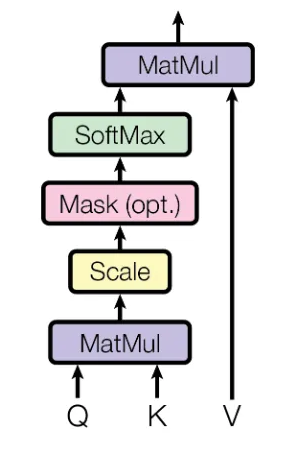
- MatMul: dot product
-
Scale: the dot product may create large values, so we scale it by dividing the output by $\sqrt{dk}$.
-
Mask: the optional padding.
-
Softmax: brings down the values to a probability distribution $[0, 1]$.
This equation is basically what the diagram above is depicting.
The scaled dot-product attention is a major component of the next part (multi-head attention).
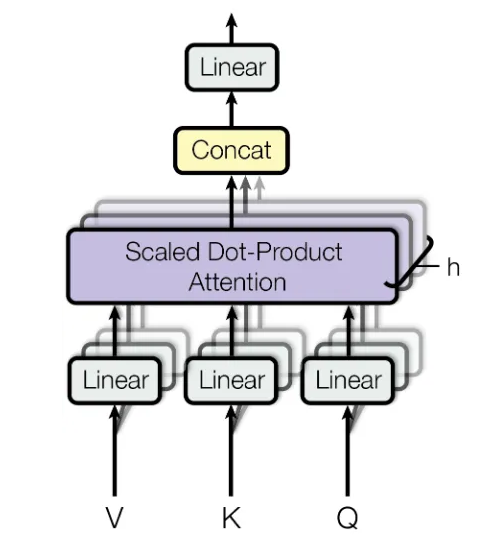
- Multi-head attention
Multi-Head Attention is essentially the integration of all the previously discussed micro-concepts. $h$ is the number of heads: the inputs to the multi-head attention are split into $h$ parts, each having Queries, Keys and Values, for max_length words in a sequence, for batch_size sequences. The dimensions of Q, K, V are called depth which is calculated as follows:
\[depth = d_{model} // h\]This is the reason why d_model needs to be completely divisible by h. So, while splitting, the d_model shaped vectors are split into h vectors of shape depth.
These vectors are passed as Q, K, V to the scaled dot product, and the output is ‘Concat’ by again reshaping the h vectors into 1 vector of shape d_model. This reformed vector is then passed through a feed-forward neural network layer. Basically divide the usual input in $h$ parts and passing them to the scaled dot product attention transformation we saw earlier.
Attention Layers are used as the basis unit in the model. Each contains an Attention Layer and a Normalization Layer and Add Layer. They’re identical except for how attention is configured.
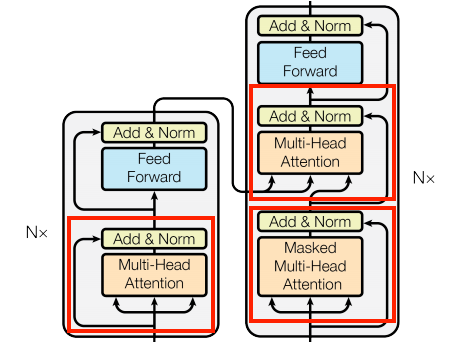
The Point-wise feed-forward network block is essentially a two-layer linear transformation which is used identically throughout the model architecture, usually after attention blocks.
For Regularization, a dropout is applied to the output of each sub-layer before it is added to the inputs of the sub-layer and normalized.
The architecture of a Transformer is now complete:
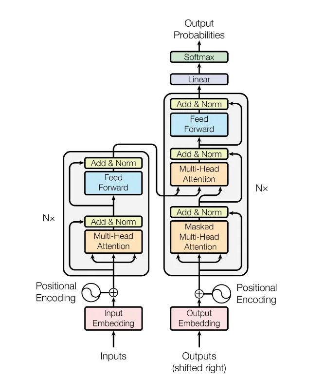
The Encoder is the part in the left and Decoder is on the right.
Attention Weights
The attention weights are visualized using heatmaps. Let’s break down the interpretation of the heatmap’s x-axis and y-axis:
-
X-axis: The x-axis represents the encoder timestep. In the context of attention mechanisms, it corresponds to the positions or steps in the input sequence (encoder) that the decoder pays attention to. Each tick on the x-axis corresponds to a specific timestep or position in the encoder sequence.
-
Y-axis: The y-axis represents the decoder timestep. It indicates the positions or steps in the output sequence (decoder) that receive attention from the encoder. Each tick on the y-axis corresponds to a specific timestep or position in the decoder sequence.
By visualizing the attention weights as a heatmap, you can observe how different parts of the input sequence (encoder) and output sequence (decoder) interact and contribute to the generation of each word in the summary. The intensity of the heatmap at a particular position indicates the strength or magnitude of attention between the corresponding encoder and decoder timesteps.
I am thus plotting the attention weights in heatmaps. Now I got a grid of plots with 8 columns representing the 8 heads in the multihead model and $N$ rows representing the amount of steps the prediction loop takes. However, in this loop I always take the attention weight corresponding to the decoder layer 4 and its block 2. What does that mean?
-
Each block in the decoder has 8 heads, since we configured the model to have 8. The use of multiple heads in the attention mechanism allows the model to capture different types of information or patterns from the input sequence simultaneously.
-
Each of the 4 layers we configured, has 2 blocks. In the original transformer model, each layer consists of two sub-layers: the multi-head self attention mechanism and the feed-forward network. Each block consists of a self-attention mechanism and a feed-forward neural network. By having multiple blocks, the model can perform multiple rounds of attention-based computations.
-
The
EncoderLayerhas one block, and eachDecoderLayerhas two blocks. Therefore, if you have fourDecoderLayerinstances, you would have a total of eight blocks in the decoder.-
The terms “block” or “block1” and “block2” are not referring to separate blocks within the layers. They are being used to indicate different attention mechanisms within the same layer. The term “block” does not refer to a separate block or layer in the model architecture.
-
The
EncoderLayerhas one multi-head attention mechanism (self.mha), and theDecoderLayerhas two multi-head attention mechanisms (self.mha1andself.mha2).
-
Technicalities I Should Know By Now
MatMul
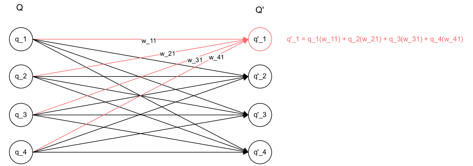
The multiplication of either $Q \times W$, $K \times W$ or $V \times W$ is often called a linear transformation because it can be expressed as a matrix multiplication, fundamental of linear algebra.
The matrix $W$ contains the learnable parameters of the layer and determines how the input $Q$ will be transformed. The weights are initialized randomly at first.
Mathematically, let $Q$ be a row vector - which is a speciall case of a matrix - of size (1, d_model):
where $dmodel$ is the number of dimensions the word embeddings have (or the number of neurons in the input layer). Then, the weight matrix $W$ has a size of (d_model, d_model). For example, if $dmodel = 4$, the linear transformation would look like below.
The linear transformation is called linear because it’s a linear combination of input $Q$ with the weights $w_{ij}$. Each element of $Q’$ is now obtained by the weighted sum of the elements in input $Q$. This is a linear operation because it involves only addition and scalar multiplication.
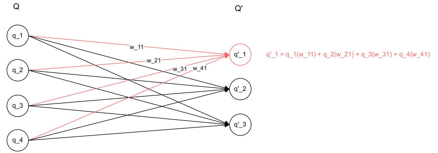
In Feed Forward Networks,
Each column of weights in weight matrix W, corresponds to the weights of one neuron in the subsequent layer.
What if we had 3 neurons in the next layer? In that case, we know that $W$ would have 3 columns and 4 rows. Therefore the multiplication would have dimensions (1, 4) x (4, 3) = (1, 3):
We can see that each the weighted sum stays the same for the remaining neurons, and by having three, we just implied we took out one row of weighted sums.
Let’s consider another example: $Q$ is a row vector with shape (1, d_model) representing the output from the previous layer (i. e., a Multihead Attention Layer). Then, $W$ is the weight matrix with shape (d_model, dff) where dff is the number of neurons in the subsequent layer.
After the matrix multiplication $Q \times W = Q’$, the resulting output will be a row vector of size (1, dff).
Dropout
Deep learning neural networks can fall into overfitting, and one of the simplest ways to avoid it is using different model configs, but it requires computational power to train each one. Thus, dropout came about: it is a way in which a single model can be used to simulate having a large number of different network architectures by randomly dropping out nodes during training.
Dropout is a regularization method that approximates training a large number of neural networks with different architectures in parallel.
By ignoring a random layer output, we make the layer look like it has a different number of nodes. This makes that, with each update during training, the network uses a different architecture. The dropout of a layer output involves removing its incoming and outgoing connections.
This is reminiscent of the last section’s second example where we stated what would happen if instead of 4 neurons in the second layer we had just 3: by removing all its connections (incoming and outgoing), the algebraic implications are basically none, since mathematically the resulting vector has one less element and the computation’s algorithm stay the same.
An example in the Transformer architecture can be seen at the Encoder Layer structure:
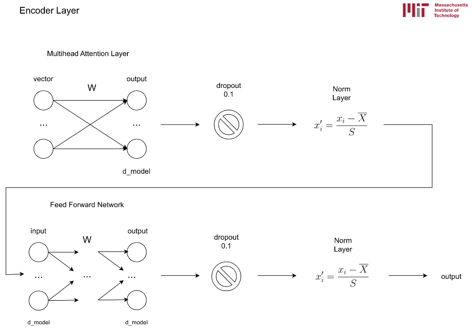
which is implemented as:
# init method
self.dropout1 = tf.keras.layers.Dropout(rate)
# call method
attn_output, _ = self.mha(x, x, x, mask)
attn_output = self.dropout1(attn_output, training=training)
If we mentioned that the dropout happens inside the layers of neurons, why would it be a separate layer? The Dropout layer is not part of the MultiHeadAttention layer because the output of the multihead attention layer is the one that goes through dropout, allowing for more control in the dropout application.
What Exaclty is Query, Key and Value?
The Q, K and V are the input to the self attention mechanism, which is used in this line:
attn_output, _ = self.mha(x, x, x, mask)
which triggers the __call__ method inside the MultiHeadAttention class:
def call(self, v, k, q, mask):
    batch_size = tf.shape(q)[0]

    # applies the layer to the params: matmul between q and the weights in the layer (learned)
    q = self.wq(q)
    k = self.wk(k)
    v = self.wv(v)

    # splits result into h parts
    q = self.split_heads(q, batch_size)
    k = self.split_heads(k, batch_size)
    v = self.split_heads(v, batch_size)

    # applies attention to each h part
    scaled_attention, attention_weights = scaled_dot_product_attention(
        q, k, v, mask)

    scaled_attention = tf.transpose(scaled_attention, perm=[0, 2, 1, 3])

    # concat the h parts again into its original shape
    concat_attention = tf.reshape(scaled_attention, (batch_size, -1, self.d_model))

    # linear step again
    output = self.dense(concat_attention)

    return output, attention_weights
But, what exactly is the Q, K and V if I’m sending the vector $x$ every time? They stand for Query, Key and Value, respectively. They are three different linear projections of the input $x$ to be used in the attention mechanism. The input $x$ is used for all three components of attention, namely the Q, K and V. This makes the algorithm pay attention to different parts of the input $x$.
Given the input sequence $x$, the Multi-head Attention performs three different linear projections of $x$ to obtain q, k, and v. These projections are performed using three separate weight matrices: wq, wk, and wv, which are the matrix multiplications of Q, K and V and a learned weight matrix. Mathematically, the projections are:
Here, $x$ is the input sequence and $W_q$ is a learned weight matrix. The multiplication means that each position in the input sequence $x$ is multiplied element-wise by the corresponding row of the matrix $W_q$. The result is the $q$ vector, which represents the query. Similarly, key and the value are obtained.
After obtaining Q, K and V, the attention mechanism computes the attention scores between the query Q and the key K to determine how much each position in the input sequence should attend to other positions. These attentions scores are computed using the scaled dot-product attention mechanism:
attention_scores = softmax((q * k^T) / sqrt(d_model))
But how would a scaled dot product output attention scores exactly, which would determine the importance of each position in the input sequence to other positions?
- We compute the scaled dot product of queries Q and keys K:
Here, $q$ and $k$ are matrices , where each row represents a query vector and a key vector. The dot product operation between them computes the similarity between each query and each key. How is this possible? Well, remember two vectors that point to the same direction and have the same length output a dot product of 1, which makes the dot product a measure of similarity!
- Then, we scale the dot product by the square root of the dimension of the query vectors $dmodel$:
This step scales the dot product from getting too large, in order to stabilize the learning process. The scaling factor $\sqrt{dmodel}$ is empirically found to work well.
- After that, we apply the softmax function along the last axis (axis=-1)
These attention scores are then used to weight the value V at each position, producing the weighted sum of values (matmul) as the attention output:
attention_output = attention_scores * v
These attention outputs from all the heads are concatenated together and linearly transformed by another weight matrix to produce the final output of the Multi-Head Attention mechanism.
q, k, and v are not three separate linear projections of x, but rather, they are derived from x through linear projections using different weight matrices.
Handy Links
-
https://blog.floydhub.com/gentle-introduction-to-text-summarization-in-machine-learning/
-
https://medium.com/swlh/abstractive-text-summarization-using-transformers-3e774cc42453
-
https://blog.jaysinha.me/train-your-first-neural-network-with-attention-for-abstractive-summarisation/
-
https://towardsdatascience.com/transformers-explained-65454c0f3fa7
-
https://www.tensorflow.org/text/tutorials/transformer
-
https://github.com/rojagtap/abstractive_summarizer/blob/master/summarizer.ipynb
-
https://medium.com/luisfredgs/automatic-text-summarization-with-machine-learning-an-overview-68ded5717a25
-
https://towardsdatascience.com/attention-and-transformer-models-fe667f958378